Objectives
The main objective is to speed-up the calibration of complex exotic models by off-loading the expensive calculations to the training phase, allowing for very fast daily calibration.
We are currently working on the training of ANNs to reproduce the SABR formula, following principles and ideas developed in McGhee.
Our latest trained ANNs can be dowloaded here, with a Jupyter notebook to test the results against Hagan’s closed-form for SABR.
The preliminary results are encouraging, as we can observe very good fits at least within the range of parameters where the ANN was trained.
Introduction
The usage of Artificial Neural Networks (ANNs) for calibration was illustrated in Hernandez where an ANN is used to replace the calibration of the Hull-White parameters by optimization on closed-form. This is an example of what we would call “Calibration Mode”, where the inputs to the ANN are market prices and the outputs are the model parameters. This has the great advantage of entirely skipping the optimization process, but has the drawback of not allowing the pricing of vanilla options with the network.
In McGhee, the ANN is used in the reverse direction, which we would call “Closed-Form Mode”. The inputs are model parameters and the outputs are market prices (or implied volatilities). The advantage in this mode is that we can value vanillas with the ANN, while of course the drawback is that calibration must go through an optmization on the ANN. Still, evaluation of the ANN may be much faster than a closed-form, and one may consider, at least in principle, training two networks, one in each direction.
Our interest in the subject is to ultimately allow for a much wider range of model choices without being limited by the need of a closed-form for calibration purposes. The process would go as follows:
- Generate random scenarios for model parameters and calculate the prices of vanilla options using an accurate numerical method (exact closed-form, PDE or Monte-Carlo simulation)
- In Calibration Mode (resp. Closed-Form Mode), train the network by taking the market prices (resp. model parameters) as inputs and model parameters (resp. market prices) as outputs
- Store the weights of the network
This process would need to be done only at sparse intervals such as every couple of months, with minor re-training when new patterns are observed in the market, typical levels have changed, etc…
Daily, the ANN produces the model parameters directly given the new market prices (in Calibration Mode), or is used to optimize to the market prices (in Closed-Form Mode). Even in Closed-Form Mode, we may expect significant speed-ups for complex models as the ANN would (hopefully) be much faster to evaluate and potentially more accurate than a complex numerical closed-form.
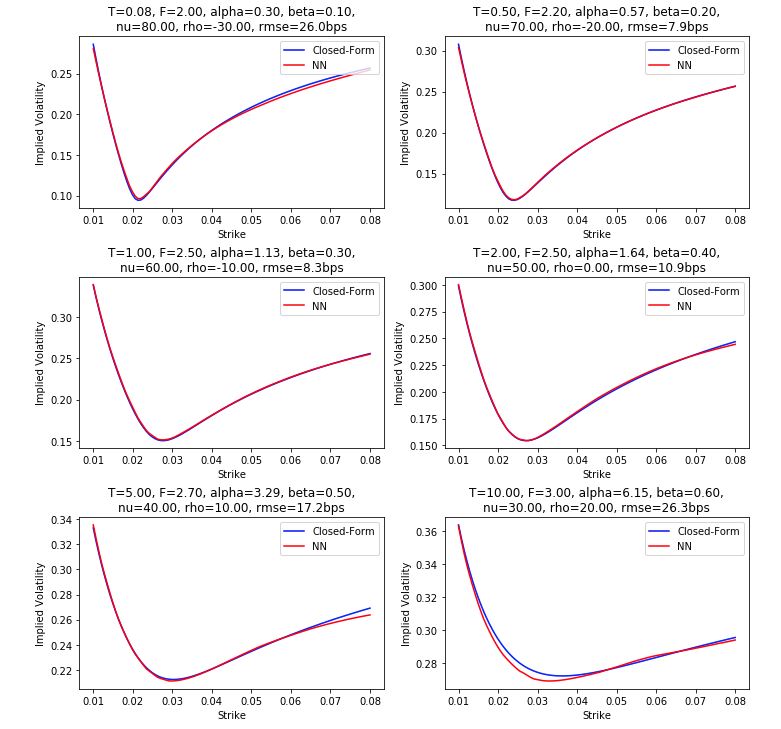
Preliminary Results
Our goal here is ultimately to use the ANN to replace numerically challenging calculation processes for SABR extensions such as Arbitrage-Free SABR, Free-Boundary SABR or ZABR.
We are starting by the standard SABR model whose implied volatility is calculated by Hagan’s formula. With inspiration from the work of McGhee, we train our networks with randomly generated SABR parameters to reproduce Hagan’s formula.
We find the good results above with a rather large range of parameters including non-trivial beta. For more information, these results were obtained by training on 800,000 samples in the following ranges
- alpha = [5%, 25%] / Fwd^(beta – 1)
- beta = [0.10, 0.80]
- nu = [20%, 80%]
- rho = [-40%, 40%]
- Fwd = [2%, 4%]
- Strike = [1%, 6%]
- T = [1M, 5Y]
The network and hyper-parameters were:
- 64 neurons per hidden layer
- 3 hidden layers: relu, softmax, relu
- Adam optimizer, learning rate 0.001
- batch size 10, 20 epochs
resulting in a training runtime of about 40 minutes in single thread.
Unsurprisingly, accuracy is maximum when testing well inside the training range and deteriorates near the edges. In particular in the chart above, the worst error is observed at T = 10Y which is outside of the training range (up to 5Y).